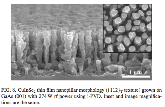
 For a while now I’ve been dying to share some of the new nanostructures I’ve discovered during ion-assisted vapor deposition of CI(G)S thin films. My paper was published in the Journal of Applied Physics last fall (sorry for the blog outage over the winter-break). The paper is titled: “Nanostructured light-absorbing crystalline CuIn(1–x)GaxSe2 thin films grown through high flux, low energy ion irradiation;” http://dx.doi.org/10.1063/1.4823987. There are a lot of unanswered questions about the work that leaves me dreaming up different solutions to how these films are growing. Read More
Work
My New Nanostructured CI(G)S Light-Absorbing Thin Films Published in JAP
March 4, 2014 – 5:06 pm
Simple Matlab Gui Programs for Crystal Symmetry Calculations
July 14, 2011 – 6:04 pm
 I’ve made a few small gui programs (MATLAB) for finding all unique angles for vectors (or plane normals) in both the cubic and tetragonal crystal spaces. I thought I’d share them here, as I finally worked out a few kinks. Be aware that the little gui’s use the command window to output their results. Some of my other programs would output latex code so that they could be pasted directly into a thesis for tables etc., but this one just uses the standard out (ala the command window in Matlab).
Essentially you enter the vectors for the two planes of interest, then hit calculate, and all the unique angle solutions for the crystal space you chose (one gui for each crystal space right now- no interest in complicating it by combining at this time) gets output in the command window.

I populate some orientation matrices based upon the vectors you give. Then, from matrix calculations, using tetragonal and crystal symmetry operations, we determine all the symmetric orientations. Then, a simple subspace() command gives us the angles of greatest rise (dihedral angle) between the symmetric orientations. The calculations for these operations can be found in my Thesis (if it ever gets published), but can also be found in: V. Randle and O. Engler. Texture Analysis: Macrotexture, Microtexture & Orientation Mapping. CRC Press, 2000.
Please note- it’s your job to check if these are correct, I make no warranties about this stuff. ![]() It should work, but feel free to go in and edit everything to your liking. If you use my code, don’t worry too much about citing me (if you do, I appreciate it, but I often leave out others who have contributed also).
It should work, but feel free to go in and edit everything to your liking. If you use my code, don’t worry too much about citing me (if you do, I appreciate it, but I often leave out others who have contributed also).
These are very simple, but hopefully they’ll help a bit for those working in cubic and tetragonal spaces.
Here’s the cubic symmetry angle calculator:
Vector Angle Calculator Cubic SymmetriesHere’s the tetragonal symmetry angle calculator:
Vector Angle Calculator Tetragonal Symmetries
I hope they work for you- please let me know if you have problems, if I have time I’ll try and help.
Finally- Qspace mapping success!
November 13, 2010 – 10:15 pm
 I have no idea why this took so long, but I finally have the code to import and output various graphs of the reciprocal space maps (RLM or Q-space) taken using the Xpert Xray diffraction system. One of the difficulties in outputting the older data has been solved by our new line-scan detector system. The data is now taken in the more simple Omega-2Theta space instead of Omega-Omega2Theta space. With the help of Mauro Sardela, the fantastic research scientist who runs the XRD lab at the Materials Research Laboratory (FS-MRL), I’ve properly translated the data into Q-space using the same equations the Xpert Epitaxy software uses.
Read More
Software For Scientists: Awk (& OsX)
October 13, 2010 – 12:45 pm
 For years while Apple had proprietary system software, I was itching to get a Unix system underneath and have the ease of the windowing system. Well, after OsX was released, I was ecstatic. Why? Because of the ease of some tasks in Unix in comparison to other OS’s. This post is only one example of what you can do if you do a bit of research into how to use your Mac. For those who have un*x boxes, this will merely be a place-holder for a few AWK scripts for you.
Read More
More on XRD Q-space mapping.
September 30, 2010 – 9:54 am
After some new scans, it appears the XRDMLread.m function I talked about is doing a pretty good job of getting the 2-axis scans into MATLAB. I was able to alter the code to accept the standard Epitaxy software’s translation to Q-space. (In Epitaxy the default is R = 0.5 I believe.) So, the following image was imported with XRDMLread.m the plotted with the standard 2-d example from the author’s website. The code was altered to output 10000xRLU units the same as Epitaxy (Panalytical). I haven’t checked all the numbers, but it’s looking ok so far. Unfortunately the color-scale looses it’s meaning as far as intensity is concerned, it appears at first glance.
 Qspace map")
Working a bit with my old q-space map code, I’m able to accomplish the following:


Note the strange love-handles the data gains. I suspect this might be due to the Gridfit function (see MATLAB files repository) I used for regridding the data. Gridfit.m uses an extrapolant method. My suspicion is it is trying to fill out the square of the data matrix and is accomplishing relatively correct values for near-by-data that is outside the scanned range. I’ll try it again with regrid or something similar in the future when I have time.
If anyone knows where the current site for XRDMLread.m is, I’d love to link to it. It appears the site may be down (graduated student I suspect). You can obtain the wonderful XRDMLread.m function and examples on the XRDMLread.m website. For now, I have to wait until I hear from the authors before I can share the file. I also don’t yet trust my icky 3D code, so I prefer not to release that until I have things hashed out. Sorry!
I’m extremely happy that Panalytical has published their XRDML file format and that the makers of XRDML.m have released their .m files for MATLAB. In the past, when Philips had the Xpert systems, the data was stuck for the most part in proprietary data formats. [You could slice the data and output in ascii- but making that work was a pain- which is why I never released that previous code.] I’m much closer to the 3d plotting now, and hope to finish it up before the thesis (my primary work which is not this plotting) is published.
Wishing you luck in you research!
Adaptive Lenses
August 31, 2010 – 9:34 am
 Every once in a while a simple solution gracefully solves a problem that affects a large number of people. It doesn’t happen often, but when it does, it’s wonderful to see the results. This is the type of thing most scientist hope to experience at least once in their careers. I think most of us at one point in time have hoped: “please let me improve the world in some small way to make life easier for some people.”
I have to admit as a scientist I love to see graceful solutions to any problem. Prof. Josh Silver at the University of Oxford has come up with just such a brilliant simple solution that any scientist who understands index of refraction will say: “Ahhh… yes!” about. Prof. Silver has made plastic glasses with adaptive lenses for third world countries. In third world countries to get glasses right now you have to either already know (by magic) your prescription, or try and somehow happen across an optometrist (and you thought it was just about affording a roof over your head!). Unfortunately, optometrists don’t grow on trees in third world countries, and so you’re pretty much out of luck.
Enter the “dial a prescription” solution of Prof. Josh Silver’s. With his glasses you simply turn a few dials which push plungers in or out of a syringe attached to each lens. These syringes hold a fluid which has the same index of refraction as a polymer film which flexes under pressure (positive and negative pressure). This pressure of course will bow out or bow in the surface of the “lens” (which is fixed on the edges to a certain thickness). How to know your prescription? Simple- is it clearer or not? [Much like the old A or B, A or B, A or B, 1 or 2, 1 or 2 hassle we all go through at the optometrist's office- but cut out all that binary testing... just dial it in or out- bam, there's your prescription- in fact, it's fractions of diopters even- so it's much more analog than the current system.] Pure brilliance. Such a simple problem to a complex issue.
The impact to those who can’t see? Huge! I suggest it’s almost as huge as teaching someone how to farm. People are illiterate because they can’t see things clearly enough to learn how to read or write. Prof. Silver’s solution has the possibility of changing all of that.
So, my hat is off to him as a scientist- excellent work, and much needed work!!
Here are some links to the adaptive lenses:
- Guardian: Inventor’s 2020 vision: to help 1bn of the world’s poorest see better
- Prof. Josh Silver’s Organization: Center For Vision In The Developing World
And here are some talks that highlight these new adjustable lens glasses:
If you’ve been moved by this simple idea, consider sending a donation to them to help support vision for those around the developing world: Donate.

Matlab doesn’t open two windows? – Here’s a fix.
June 29, 2010 – 10:11 am
After finally installing Leopard (10.5) osX on my Powerbook G4 (Thesis writing computer), I noticed a strange behavior with MATLAB. MATLAB could no longer open more than one instance of itself. As well, it could no longer open a window once it had opened once in any login session. Strange behavior indeed.
Well, here’s the fix… it turns out that Leopard uses launchd to set the display. So, the old method of launching MATLAB was to set the display to 0.0, but this will fail after the first instance, hence the bug. What you can do is simply remove this line from the startup script in matlab (located within the startup application contents).
The line that was:
$SHELL -c 'bin/'$ARCH'/setsid bin/matlab -desktop -display :0.0 &'
should now be:
$SHELL -c 'bin/'$ARCH'/setsid bin/matlab -desktop &'
Once I changed that, everything started up fine! ![]()
ps- you will know you have this problem if you look at your console log immediately after launching MATLAB and it says something like:
6/29/10 9:03:34 AM [0x0-0x78078].StartMATLAB[23469] Warning: Unable to open display :0.0, MATLAB is starting without a display.
NY-PBS Captures The Struggle Of The Graduate Student
April 9, 2010 – 12:52 am
It’s not often that someone goes about deciding to make a film about graduate studies. It just so happens that Thirteen (PBS-NY) has done just that. Their film “Naturally Obsessed: The Making Of A Scientist” is quite an excellent snap-shot of the struggle of graduate students to get their PhD degree and accomplish something very difficult. Of course each of our struggles is unique. We are all dealing with our own situations, with our own fields (some not even in laboratories- the horror- is that real science? hahahah).
Speaking of our own struggles, what most of the public often does not get a feel for is the absolute devotion, almost to insanity, towards finding the solutions we are looking for. Many of the comments by the graduate’s spouses touched home for me. In each of the graduates followed in this film I saw bits of myself. One thing however, that is different, is the struggle for the specific protein structure. Often that struggle is a lot less well-defined. In this situation, you either get the structure of AMPK or you don’t. I guess it’s a lot like their attempts at creating crystals. Sure, you get crystals, but if they don’t have a periodic structure, you’ll never get diffraction. In my situation, the variables in our studies are very difficult to control, and so often one doubts one’s work solely on the question of reproducibility. Many scientists struggle with this same situation. People think that doing things like “measuring temperature” is a very easy thing. In reality, it is a very very difficult thing. Especially in a vacuum. ![]() That question just arose the other day in discussing our science with a new undergraduate assistant. As we talked more and more on the difficulties of measuring temperature we all saw his eyes grow larger in wonder. The simplest of problems can often be the most difficult. How accurate do you need to measure it? What standard will you use? Do you believe your thermocouple, your thermometer, or your pyrometer? What if the emissivity of the surface changes?
That question just arose the other day in discussing our science with a new undergraduate assistant. As we talked more and more on the difficulties of measuring temperature we all saw his eyes grow larger in wonder. The simplest of problems can often be the most difficult. How accurate do you need to measure it? What standard will you use? Do you believe your thermocouple, your thermometer, or your pyrometer? What if the emissivity of the surface changes? ![]()
This is the life of a scientist. And the film below attempts to capture the lives and struggles of a few graduate students who are hoping for a career in science. It’s a struggle. But, you have heard me say that enough. ![]() To learn more about it I strongly suggest you watch this film. For the graduate student, I warn you: you’ll see yourself in this. For those who aren’t scientists: this may end up being a comedy, and I kindly refer you to Marg Simpson’s commentary on graduate students posted earlier in this blog.
To learn more about it I strongly suggest you watch this film. For the graduate student, I warn you: you’ll see yourself in this. For those who aren’t scientists: this may end up being a comedy, and I kindly refer you to Marg Simpson’s commentary on graduate students posted earlier in this blog.
My congratulations to Thirteen for doing such an excellent job on this one hour film. They didn’t have a lot of time to share with you everything regarding our struggles and achievements, but they distilled it quite well in the time available.
Prof. Janice Tomasik – Chemistry Education
September 14, 2009 – 12:28 pm
 My sister, Janice, got a great mention in C&E News! She is a professor at Central Michigan University in Chemistry. Her studies and research are in Chemistry Education. Read More
MATLAB and reciprocal space mapping – small update.
June 24, 2009 – 2:07 pm
Well, I’m one of those guys who believes a picture is usually worth a ton of words. I’ve got a few images to share here on the matlab code I’ve been working on for reciprocal space mapping in MATLAB. I’m still not 100% on my code right now, so I’m not sharing it for the time-being. In particular, I use an import function for .x00 slices for two-axis scans in the Panalytical/Philips XPert system. If you are using XRDML, skip the files for .x00 import that I have in other posts on this blog. In anycase, without much explanation here are the images…


-
Work Categories
-
Archives
-
More of Me
-
Intranet

